P95 and P99 highlight slow requests that might otherwise be masked by an average value. A P95 In simple terms, this describes the duration that approximately 95 percent of the selected requests do not exceed. The meaning behind this depends on the measurement point, the time period, and the number of requests recorded. Histograms provide estimates for this, the accuracy of which depends on their resolution. For a reliable operational view, query volume and error rate must also be included; a percentile alone explains neither the cause of a delay nor the experience of individual users.
What Latency Measurement Captures
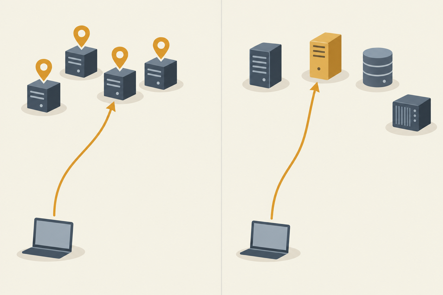
A latency metric is only meaningful if you Measuring point It is clear that a reverse proxy can measure the duration of a request as it passes through the proxy to the service; an application, on the other hand, measures a segment within its own processing. The specific steps included depend on where the measurement begins and ends.
A measurement taken in the browser can also capture parts of the path between the client and the server, as well as client-side processing. Here, too, the specific instrumentation determines the start and end points. Low server latency alone therefore does not prove that a page is quickly usable in the browser: network transmission and processing on the end device can take additional time.

Also place the Population Note: Does this apply to all requests for a service or to a specific endpoint? The overall distribution may differ from that of a single endpoint. Also note whether the analysis covers a five-minute rolling window or a longer period, and whether the values are displayed in seconds or milliseconds.
Successful and failed requests are also included in the definition. An error returned quickly can improve the latency distribution, even though the request did not reach its destination. Separate views for success and failure help identify these cases; additionally, the error rate remains a standalone operational metric.
The OpenTelemetry convention in the development branch specifies a histogram of request durations in seconds for HTTP servers. This does not mean that a specific installed version supports it or exports it under the same name. Check the actual metric name and available attributes in your environment before building a dashboard around it.
How to Read P95 and P99 Correctly
A Percentile describes a boundary within the selected distribution. If P95 is 400 milliseconds, then—to put it simply—about 95 percent of the request durations considered are no longer than that. P99 shifts the focus further toward the slower end: It describes the boundary for about 99 percent of the observations.
| Key figure | Statement | Limitations of the Statement |
|---|---|---|
| average | Sum of durations divided by the number of requests | Hides the distribution of individual fast and slow requests |
| P50 | Threshold for approximately half of the observed durations | Does not describe how slow the upper end is |
| P95 | Threshold for approximately 95 percent of the observed durations | Slower observations above the threshold remain invisible as a single value |
| P99 | Threshold for approximately 99 percent of the observed durations | With only a few observations, the result may depend heavily on individual values |
These percentages are based on measured values, not directly on individuals or sessions. One person may trigger multiple requests, while another may send only one. Therefore, a P99 value alone does not indicate that one percent of users experienced a slow session.
The exact boundary also depends on the calculation method. When measurement values are identical, or when the desired position lies between two observations, different quantile definitions may select or interpolate values differently. In the case of estimated histogram values, the division into buckets must also be taken into account; therefore, a displayed value is not always an actual observed individual duration.
For hosting monitoring, the percentile includes the request volume and the error rate. The same P99 value must be interpreted differently when there are few requests versus when there are many; without volume data, it is difficult to assess its stability. The error rate also highlights an aspect that a simple duration distribution does not reliably capture.
How Histograms Estimate Percentiles
A classic Prometheus histogram does not store a sorted list of all request durations. It counts observations in cumulative buckets: A bucket with a specific upper limit also includes observations that are already in lower buckets. These counts can be used to estimate the range of the distribution within which a given percentile lies.
Suppose the position we are looking for lies between 200 and 500 milliseconds. The histogram shows how many observations were counted up to these limits, but not their exact distribution within that range. For classic histograms, Prometheus estimates the position within this bucket using linear interpolation.
This estimate may differ from the actual individual values. In particular, a broad bucket centered around a threshold value that is important for operations leaves considerable room for uncertainty: the observations within the range could be distributed differently than assumed in the interpolation. Tighter limits in relevant ranges improve resolution but require additional data collection.

Native histograms use a different representation than traditional bucket time series. Their quantiles are also estimates; the Interpolation It depends on the schema and bucket used. Classic and native histograms should therefore not be treated as if they had the same storage and always used the same interpolation rules.
Quantile can calculate a summary directly within the instrumented process. However, these individual quantile values cannot be combined retrospectively to form a correct overall quantile for multiple processes. For a joint analysis across instances, aggregatable histogram data is therefore often the more suitable basis; the bucket boundaries must correspond to the desired aggregation.
When the Average Hides Outliers
Illustrative calculation example, not a measurement: Within a given time window, 95 requests each take 100 milliseconds, and five additional requests each take 2,000 milliseconds. All 100 observations belong to the same selected population. This example is intended to compare metrics and does not serve as a performance benchmark for a hosting system.
For the percentiles, we use a specific Selection Rule: The goal is to find the smallest observed value for which at least the specified percentage of requests falls at or below that value. When sorted, the list initially contains 95 values of 100 milliseconds, followed by five values of 2,000 milliseconds.
| Key figure | Calculation or Selection | Result |
|---|---|---|
| average | (95 × 100 ms + 5 × 2,000 ms) / 100 | 195 ms |
| P95 | 95. sorted value | 100 ms |
| P99 | 99th sorted value | 2,000 ms |
The average is significantly shorter than the duration of the five slow queries. It distributes the additional time from those queries mathematically across all observations. Therefore, if one considers only this value, one cannot determine either the duration of the slow queries or, at a glance, how many of them are affected.
P95 is 100 milliseconds here, even though 5 percent of the requests take 20 times as long. The slow observations lie just above the selected P95 threshold; P99 makes them visible in this example. This does not mean that P99 generally captures every relevant delay.
Other definitions of quantiles may interpolate between sorted values and thus yield different results. Even a percentile estimated from histogram buckets may not match the selection based on individual values. Therefore, when interpreting the displayed value, one must consider the calculation method, the number of queries, and the time window under consideration.
Querying P95 with PromQL
For the following query, you'll need access to a Prometheus data source and an actual classic histogram for request durations. Enter the expression in the Prometheus expression browser or in a Grafana query field for Prometheus. The query reads existing time series; it is neither a terminal command nor a configuration change.
The metric name is a placeholder. Replace it with the name of your instrumentation if necessary, and verify that the selected time series have compatible bucket boundaries. The example aggregates across all remaining labels without additional filters and therefore returns the desired total value only if this selection matches your operational query.
First, calculate rate from the cumulative bucket counters, their rate of change over the five-minute moving window. Then, it adds sum by (le) the rates across the other labels. This order makes it possible to account for counter resets in individual time series when calculating the rates.
The Label le remains unchanged: It denotes the upper bound of the respective bucket. From the aggregated distribution, we estimate histogram_quantile the Total P95. Since we are using a metric based on seconds here, the result is also given in seconds; 0.4 therefore corresponds to 400 milliseconds.
For P99, replace the first parameter 0.95 through 0.99. For example, you can use appropriate label filters to select a service; additional grouping labels allow you to separate the results. Check in each case which queries are included and whether the bucket resolution is sufficient for the area of interest.
For Native histograms A different query syntax applies: You do not use the traditional separate _bucket-Series with le. Whether native histograms are available and how they are exported depends on the components and versions used.
Compare Instances and Request Groups
A combined P99 for cache hits and dynamic calls answers the question about the total selected set of requests. However, it does not explain which group has changed. If the proportion of fast cache hits shifts, the total value can also change without every single group necessarily having slowed down.
Therefore, supplement the overall value with separate views for subject-relevant Inquiry Groups, provided that appropriate labels are available. A specific route name or cache status can be useful for this purpose. On the other hand, using individual URLs or user IDs as labels can generate a large number of time series; choose dimensions that answer a specific question.
To calculate an overall percentile across multiple instances, compatible classical histograms first consolidate the bucket counts—or their rates—for each threshold. The quantile is estimated only from this combined distribution. Averaging individual instance P99 values generally does not yield a correct overall P99, because the distributions and query counts may differ.
| Data Format | Aggregation and Accuracy | Data Effort |
|---|---|---|
| Histogram | Compatible buckets can be aggregated; quantiles are estimated, and accuracy depends on resolution and display | Time series or histogram data for each selected resolution and label combination |
| Summary | Quantiles calculated during the process cannot be aggregated into a single overall quantile; accuracy depends on the configuration | Quantile Calculation in the Process and Time Series for Configured Quantiles |
| Individual events | Joint analysis is possible if relevant individual values are available; the result depends on the chosen quantile method | Potentially one data record per query; storage and analysis can be time-consuming |
A Summary can be useful for analyzing a single process. However, the quantiles calculated there cannot be combined retrospectively to form a correct quantile for all instances. Individual events allow for a different level of detail, but require that the necessary observations have actually been recorded and are available.
Set Latency Targets and Alarms
A latency target can only be verified if the population is clearly defined. Therefore, the statement „95 percent of the selected requests take no more than 300 milliseconds“ requires information about the measurement point, the endpoints involved, and the evaluation period. A five-minute window addresses a different operational question than a one-day window.
For the Threshold percentage Divide the number of observations up to and including 300 milliseconds by the total number of observations. In a classic histogram, a bucket with exactly this threshold provides the corresponding count; for a time window, you use the corresponding count changes or rates. The percentage immediately shows whether the selected threshold was reached within the window.
If there is no bucket threshold set at 300 milliseconds, the exact proportion cannot be determined from the bucket counters alone. The estimated P95 can still provide a rough guide, but its accuracy depends on the distribution and the bucket thresholds. For a critical threshold, it is therefore worth checking the histogram configuration in advance.
Also, explicitly define how errors are factored into the metric. A quickly resolved error message should not automatically be counted as a good user experience; depending on how the metric is defined, errors may be tracked separately or classified as negative events. It is crucial that the numerator and denominator align with the chosen definition.
A Alarm duration This prevents every minor fluctuation from immediately triggering a notification. Set a minimum number of observations so that a few isolated queries do not disproportionately influence the decision to trigger an alert. Both values should be appropriate for the volume of traffic and the urgency of the service; missing data requires special handling.
In the dashboard, it is helpful to display the target percentage, request volume, and error rate side by side. This makes it possible to determine whether a target violation affects many requests or is limited to a small window of time. An alert should also indicate which selection and time period triggered the notification.
Systematically Examine Rising Percentiles
If the P99 rises, first check the query volume and the Endpoint Mix. An increase in the number of slow dynamic requests can shift the overall value, even if the duration of each individual request group has hardly changed. Conversely, a decrease in the number of fast requests can increase the proportion of slower requests.
Next, compare separate views by route and status group, provided that the instrumentation provides these labels. A notable route can help narrow down the search; separate error groups also show whether fast or slow responses are influencing the distribution. Use broad route categories whenever possible instead of individual URLs or user IDs.
Next, examine load, queues, database response time, and error rate in parallel over the same time period. A growing queue accompanied by a rising P99 is a starting point for investigation, but it is not yet proof that it is causing the delay. Also check whether the metrics pertain to the same service and comparable groups of requests.
Help with individual slow processes Traces and specifically selected logs, provided they are available and linked to the request context. For example, a trace can show which section of a request path is taking a long time. Whether this section is actually the cause must then be verified through further observations.
The article on explains how metrics, logs, and traces complement each other when addressing operational issues. Observability in Hosting. For queues, the Mail Queue Monitoring A related use case: That one deals with the delivery of messages, not directly with the latency of an HTTP request.
For each comparison, note which time windows and measurement points are involved. A simultaneous increase in database duration and server latency may warrant further investigation, but temporal correlation alone does not prove a causal relationship. Changes in traffic or instrumentation can also influence the observed pattern.
Data Quality and Operational Decisions
When traffic is light, P99 reacts strongly to individual observations. Ten requests in a single window do not allow for as stable a classification as a large volume of requests; therefore, display the number of observations next to the percentile. For alerts, a minimum threshold can help ensure meaningful results without completely excluding underutilized services from monitoring.
A empty window This does not mean there were no observed requests or that latency was zero milliseconds. Display missing or undefined values appropriately in the dashboard, and determine separately whether the absence of traffic is itself a problem. This prevents a lack of data from being mistakenly interpreted as an exceptionally fast response.
Time periods also cannot be aggregated arbitrarily: A five-minute P99 describes a different window than a daily P99. The average of individual minute-P99s generally does not yield a daily P99. For the daily analysis, you need the underlying aggregatable distribution data for the desired time period.
The Bucket Resolution This helps determine how accurately a histogram can represent the threshold of interest. More finely tuned thresholds can improve the estimate in the relevant range, but with traditional histograms, they require additional time series and thus more memory. Weigh this effort against the benefits for the specific operational decision.
For ongoing assessment, the metrics complement one another: The average describes the median duration, P95 and P99 highlight slow areas, and the threshold percentage addresses a specifically defined latency target. Request volume and error rate provide the context needed to interpret these values. No single metric can replace a review of the measurement point, time period, and data quality.
Sources and Current State of Knowledge
Status of the research:
Research based on information as of November 16, 2026; OpenTelemetry conventions from the development branch do not constitute a guarantee for installed versions.
https://sre.google/workbook/monitoring/
https://prometheus.io/docs/practices/histograms/
https://github.com/open-telemetry/semantic-conventions/blob/main/docs/http/http-metrics.md
https://prometheus.io/docs/specs/native_histograms/
https://grafana.com/docs/grafana/latest/datasources/prometheus/query-editor/